Tutorial
Installation
TransferMatrix.jl is a part of Julia's general registry and the source code can be found at https://github.com/garrekstemo/TransferMatrix.jl. From the Julia REPL, enter the package manager mode mode by typing ]. Then just enter the following to install the package:
pkg> add TransferMatrixA simple calculation
To get up and running, let's build a simple two-layer structure of air and glass and calculate the reflectance and transmittance to visualize the Brewster angle for p-polarized light. We fix the wavelength of incident light and vary the angle of incidence.
We start by making a Layer of air and a Layer of glass. We'll do this for a wavelength of 1 μm. Since there are only two layers and the transfer matrix method treats the first and last layers as semi-infinite, there is no need to provide a thickness for our glass and air layers. From the examples below, you can see that there are fields for
- the material
- the layer thickness
The material is a RefractiveMaterial from the RefractiveIndex.jl package. You can also initize a Layer with data for the refractive index and extinction coefficient.
using TransferMatrix
using RefractiveIndex

n_air = RefractiveMaterial("other", "air", "Ciddor")
n_glass = RefractiveMaterial("glass", "soda-lime", "Rubin-clear")[1]
air = Layer(n_air, 0.1)
glass = Layer(n_glass, 0.1)
layers = [air, glass];
2-element Vector{Layer}:
Layer(TransferMatrix.var"#3#4"{RefractiveIndex.RefractiveMaterial{RefractiveIndex.Gases{5}}}(RefractiveIndex.RefractiveMaterial{RefractiveIndex.Gases{5}}("air (Ciddor 1996: n 0.23–1.690 µm)", "P. E. Ciddor.\nRefractive index of air: new equations for the visible and near infrared.\n<a href=\"https://doi.org/10.1364/AO.35.001566\"><i>Appl. Optics</i> <b>35</b>, 1566-1573 (1996)</a><br>\n[<a href=\"https://github.com/polyanskiy/refractiveindex.info-scripts/blob/master/scripts/Ciddor%201996%20-%20air.py\">Calculation script (Python)</a> - can be used to calculate the refractive index of air for specific values of humidity, temperature, pressure, and CO<sub>2</sub> concentration]\n", "Standard air: dry air at 15 °C, 101.325 kPa and with 450 ppm CO<sub>2</sub> content.\n", RefractiveIndex.Gases{5}((0.0, 0.05792105, 238.0185, 0.00167917, 57.362)), (0.23, 1.69), Dict{Symbol, Any}(), Dict{Symbol, Any}(:type => "formula 6", :wavelength_range => "0.23 1.690", :coefficients => "0 0.05792105 238.0185 0.00167917 57.362"))), 0.1)
Layer(TransferMatrix.var"#3#4"{RefractiveIndex.RefractiveMaterial{RefractiveIndex.Cauchy{5}}}(RefractiveIndex.RefractiveMaterial{RefractiveIndex.Cauchy{5}}("soda-lime (Rubin 1985: Clear; n,k 0.31–4.6 µm)", "M. Rubin.\nOptical properties of soda lime silica glasses.\n<a href=\"https://doi.org/10.1016/0165-1633(85)90052-8\"><i>Sol. Energy Mater.</i> <b>12</b>, 275-288 (1985)</a>\n", "Clear soda lime silica window glass\n", RefractiveIndex.Cauchy{5}((1.513, -0.003169, 2.0, 0.003962, -2.0)), (0.31, 4.6), Dict{Symbol, Any}(), Dict{Symbol, Any}(:type => "formula 5", :wavelength_range => "0.31 4.6", :coefficients => "1.5130 -0.003169 2 0.003962 -2"))), 0.1)Now that we have our glass and air layers, we can iterate over the angles of incidence and compute the reflectance and transmittance for light of wavelength 1 μm.
λ = 1.0
θs = 0.0:1:85.0
result = angle_resolved([λ], deg2rad.(θs), layers);
TransferMatrix.AngleResolvedResult([0.04172141224054619; 0.04170461618458165; … ; 0.4265002281178984; 0.4925481784888797;;], [0.04172141224054619; 0.04173821138353588; … ; 0.6924172620222976; 0.7359391663135002;;], [0.9582785877594537; 0.9582953838154187; … ; 0.5734997718821007; 0.5074518215111196;;], [0.9582785877594537; 0.9582617886164644; … ; 0.30758273797770175; 0.26406083368649935;;])Let's now plot the result using the Makie.jl data visualization package.
using CairoMakie

brewster = atan(n_glass(λ)) * 180 / π

f = Figure()
ax = Axis(f[1, 1], xlabel = "Incidence Angle (°)", ylabel = "Reflectance / Transmittance")
lines!(θs, result.Tss[:, 1], label = "Ts", color = :firebrick3)
lines!(θs, result.Tpp[:, 1], label = "Tp", color = :orangered3)
lines!(θs, result.Rss[:, 1], label = "Rs", color = :dodgerblue4)
lines!(θs, result.Rpp[:, 1], label = "Rp", color = :dodgerblue1)
vlines!(brewster, color = :black, linestyle = :dash)
text!(35, 0.6, text = "Brewster angle\n(Rp = 0)")

axislegend(ax)
f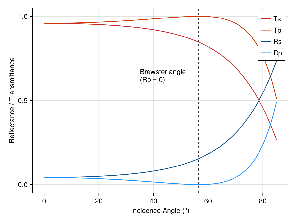
We can see that the result of the angle-resolved calculation has four solutions: the s-wave and p-wave for both the reflected and transmitted waves. And we see that the Brewster angle is $\arctan\left( n_\text{glass} /n_\text{air} \right) \approx 56^{\circ}$, as expected. Simultaneous calculation of s- and p-polarized incident waves is a feature of the general 4x4 transfer matrix method being used. The angle_resolved function will also loop through all wavelengths so that you can plot a color plot of wavelength and angle versus transmittance (or reflectance).
A simple multi-layered structure
Now that we can make Layers, we can put them together to calculate the transfer matrix for a multi-layered structure and plot the reflectance and transmittance spectra. An important structure in optics is the Fabry-Pérot etalon, made with two parallel planar mirrors with a gap between them. If we set the optical path length to be an integer multiple of half the wavelength, we get constructive interference and a resonance in the transmittance spectrum. In the frequency domain, the cavity modes are evenly spaced by the free spectral range (FSR). We will scan in the mid infrared between 4 and 6 μm and use data generated via the Lorentz-Drude model for each 10 nm-thick gold mirror. (Note that we stay in units of micrometers for the wavelength.)
caf2 = RefractiveMaterial("main", "CaF2", "Malitson")
au = RefractiveMaterial("main", "Au", "Rakic-LD")
air = RefractiveMaterial("other", "air", "Ciddor")

λ_0 = 5.0
t_middle = λ_0 / 2
air = Layer(air, t_middle)
au = Layer(au, 0.01)
layers = [air, au, air, au, air];

λs = range(2.0, 6.0, length = 500)
frequencies = 10^4 ./ λs

Tp = Float64[]
Ts = Float64[]
Rp = Float64[]
Rs = Float64[]
for λ in λs
    Tp_, Ts_, Rp_, Rs_ = calculate_tr(λ, layers)
    push!(Tp, Tp_)
    push!(Ts, Ts_)
    push!(Rp, Rp_)
    push!(Rs, Rs_)
end

f, ax, l = lines(frequencies, Ts)
ax.xlabel = "Frequency (cm⁻¹)"
ax.ylabel = "Transmittance"
f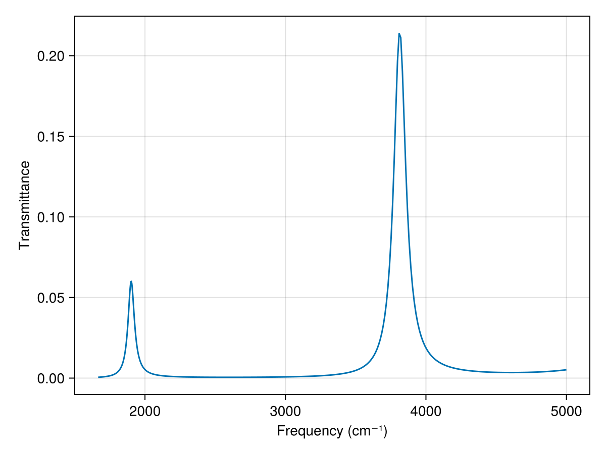
Electric field calculation
The wavelength-dependent electric field is the cavity is provided by the electric_field function. We can calculate the electric field at the first peak in the above plot using
λ_min = findfirst(λs .> 4.9)
λ_max = findfirst(λs .> 5.5)
peak = findmax(Ts[λ_min:λ_max])[2] + λ_min - 1
λ = λs[peak]

field = electric_field(λ, layers)

f, ax, l = lines(field.z .* 1e3, real(field.p[1, :]))
vlines!(field.boundaries[1], color = :black, linestyle = :dash)
vlines!(field.boundaries[end] .* 1e3, color = :black, linestyle = :dash)
f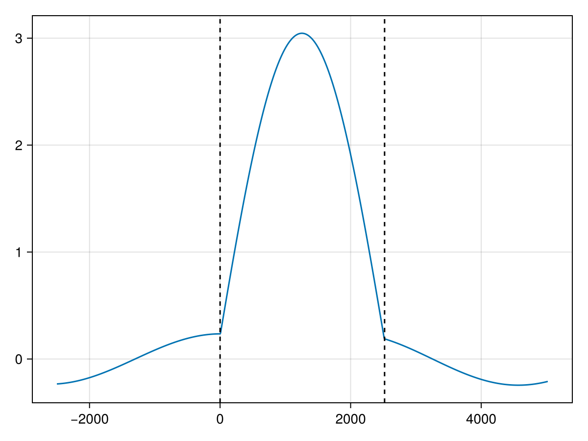
User-generated refractive index data
A convenience function is available to generate a Layer with user-generated refractive index data. For example, if we want to make an absorbing layer modeled on a Lorentzian function, we would
- Generate the dielectric function for the absorbing material.
- Calculate the refractive index and extinction coefficient.
\[\begin{aligned} \varepsilon_r(\omega) &= n_\infty^2 + \frac{A (\omega_0^2 - \omega^2)}{(\omega^2 - \omega_0^2)^2 + (\Gamma \omega)^2} \\ \varepsilon_i(\omega) &= \frac{A \Gamma \omega}{(\omega^2 - \omega_0^2)^2 + (\Gamma \omega)^2} \\ n(\omega) &= \sqrt{\frac{\varepsilon_r + \sqrt{\varepsilon_r^2 + \varepsilon_i^2}}{2}} \\ k(\omega) &= \sqrt{\frac{-\varepsilon_r + \sqrt{\varepsilon_r^2 + \varepsilon_i^2}}{2}} \\ \end{aligned}\]
where $A$ is the amplitude, $\omega_0$ is the resonant frequency, $\Gamma$ is phenomenological damping, and $n_\infty$ is the background refractive index. Then this data, along with the wavelengths and thickness of the layer, can be used to create a Layer object. Under the hood, this data is converted into an interpolation function that, when given a wavelength, will return the complex refractive index. (Extrapolation is not supported right now.)
function dielectric_real(ω, p)
    A, ω_0, Γ = p
    return @. A * (ω_0^2 - ω^2) / ((ω^2 - ω_0^2)^2 + (Γ * ω)^2)
end

function dielectric_imag(ω, p)
    A, ω_0, Γ = p
    return @. A * Γ * ω / ((ω^2 - ω_0^2)^2 + (Γ * ω)^2)
end

# absorbing material
λ_0 = 5.0
λs = range(4.8, 5.2, length = 200)
frequencies = 10^4 ./ λs
n_bg = 1.4
A_0 = 3000.0
ω_0 = 10^4 / λ_0  # cm^-1
Γ_0 = 5
p0 = [A_0, ω_0, Γ_0]
ε1 = dielectric_real(frequencies, p0) .+ n_bg^2
ε2 = dielectric_imag(frequencies, p0)
n_medium = @. sqrt((sqrt(abs2(ε1) + abs2(ε2)) + ε1) / 2)
k_medium = @. sqrt((sqrt(abs2(ε1) + abs2(ε2)) - ε1) / 2)

absorber = Layer(λs, n_medium, k_medium, t_cav)
absorber.dispersion(4.9)
A complete example calculating dispersion of a polaritonic system is provided in the examples folder of the package source code.
Thickness-dependent calculations
Instead of angle-resolved, you might want to vary the thickness of a particular layer. A convenience function, tune_thickness is provided to do this. It takes a list of wavelengths, a list of thicknesses, the layers, and the index of the layer to vary. For example, if you want to vary the 14th layer in the layers array, you might do the following:
tune_thickness(λs, thicknesses, layers, 14)A complete example using this is provided in the examples folder of the package source code.